
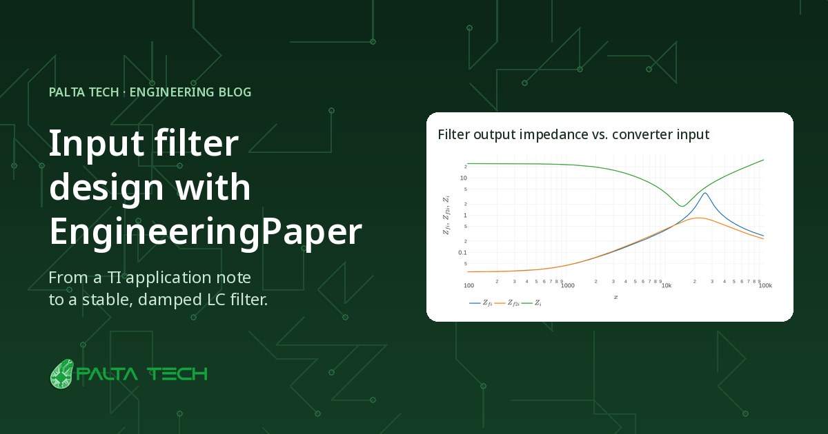
Not every switching regulator needs an input filter, but when a design calls for one, it starts with the same question: which formulas, and how do they apply to this board? At Palta Tech we answer it in EngineeringPaper.xyz. It lets us type an application note's equations almost exactly as they're printed, check our numbers against the note's, and plot the result in minutes.
By the end of this article, you'll understand:
- Why a switching supply's input filter can make the converter oscillate
- How an application note can be followed step by step, using TI's SNVA538 as the example
- How to check a filter against the Middlebrook stability criterion
- Why EngineeringPaper.xyz is our favorite tool for app-note math
Why the Input Filter Matters
An input filter on a switching power supply has two jobs:
- Keep the converter's switching noise from reaching the supply line and disturbing other equipment, which is also what conducted-EMI tests measure.
- Keep high-frequency noise already on the supply line from passing through to the converter's output.
An LC filter does both. But there is a catch. Inside its control-loop bandwidth, a regulated converter draws constant power: when its input voltage rises, its input current falls. That behaves like a negative resistance. Put a lightly damped LC filter in front of it and the two can form an oscillator. A filter that looks perfect on paper can make a working converter ring, or oscillate outright, once it's connected.
Why We Use EngineeringPaper.xyz
Hardware is hard, and a lot of that difficulty lives in the math. Before a board is built, you need equations that tell you whether a circuit will behave, and especially under which conditions it must not oscillate. Today, an engineer who designs hardware needs a tool for prototyping the equations of a specific circuit as quickly as they prototype the circuit itself.
For years, the Palta Tech team looked for an open-source application that was fast and let us write equations the way we would by hand. The tools we tried always fell short somewhere:
- Some were free to use but not open source.
- Some recalculated slowly, which breaks your flow when you're iterating on component values.
- Most made it hard to turn our engineering notes into something we could put in a user manual or a design-decision record.
EngineeringPaper.xyz ticks every box. It's open source, runs in the browser, and the support has been excellent from the very first day we started using it. There is also a paid desktop version, EngineeringPaper.pro, which we highly recommend for complex projects. It opens several sheets side by side in tabs, lets you keep each part of a design in its own sheet file and then import them into one sheet, and generates the combined DOCX or PDF report locally. Here's what it gives us:
- Math that looks like handwriting. You type and it typesets as you go: fractions, square roots, absolute values, Greek letters and subscripts.
- Fast, live results. Change one value and every result and plot below it updates.
- Plots in the sheet. Any expression can be swept and plotted with log axes, and you can overlay several curves to compare them.
- Notes that become documents. A sheet exports to Markdown, Word, PDF or LaTeX, so the same calculation goes straight into a user manual or a design review. In the free web version, Word, PDF and LaTeX files are generated on the EngineeringPaper.xyz server and carry a watermark; the paid desktop app generates them locally without one.
- Files you can keep. The native
.epxyzfile can be tracked in your normal, day-to-day hardware repository, right next to the schematic and the layout.
Same Names as the Application Note
Our favorite feature is the simplest: variable names can match the application note exactly, subscripts included. When the note writes ESRci, fcfilter1 or Z2eqi, so does our sheet. Comparing our sheet to the note becomes a line-by-line read, not a translation exercise:
| In the application note | In EngineeringPaper.xyz |
|---|---|
ESRci := 0.150Ω |
ESRci = 0.150 |
fcfilter1 := 1 / (2·π·√(Lf·Cf)) |
fcfilter1 = 1 / (2·π·√(Lf·Cf)), typeset as a real fraction |
Z2eqi := Z2i·Rin / (Z2i + Rin) |
Z2eqi = Z2i·Rin / (Z2i + Rin) |
ζ := L / (2·Rin·√(L·C)) |
ζ = Lin / (2·Rin·√(Lin·Cin)) |
The Application Note: TI SNVA538
How many of you have found this kind of treasure? Semiconductor vendors like Texas Instruments, Infineon and ST share an enormous amount of engineering knowledge for free, mostly as a long trail of PDF application notes. Analog Devices takes a different route and publishes many of its technical articles as web pages that you can also download as PDF. Either way, the knowledge is there, and an application note is often the shortest path from a blank page to a working design.
Our reference is "Input Filter Design for Switching Power Supplies" (SNVA538) by Michele Sclocchi, originally published by National Semiconductor and now by Texas Instruments. It is short, practical, and covers four filter types:
| Filter | How it's built | Trade-off |
|---|---|---|
| Undamped LC | One inductor and one capacitor | Smallest, but a tall resonance peak |
| Parallel damped | Rd in series with a blocking capacitor Cd, across the filter capacitor | Easily meets damping needs; Cd is large |
| Series damped | Rd in series with Ld, across the filter inductor | Smaller parts, but less high-frequency attenuation |
| Multiple sections | Two or more LC stages | More attenuation for the same volume and cost |
The appendix works through a complete example: a 40 V to 5 V, 1 A buck converter built on the LM2675-5.0. The note's own calculations are Mathcad worksheets. We have rebuilt that example in EngineeringPaper.xyz so you can see the potential of this kind of tool in a modern hardware workflow, where the calculations live right alongside the schematic and the PCB layout. The rest of this article walks through it.
The Design, Step by Step
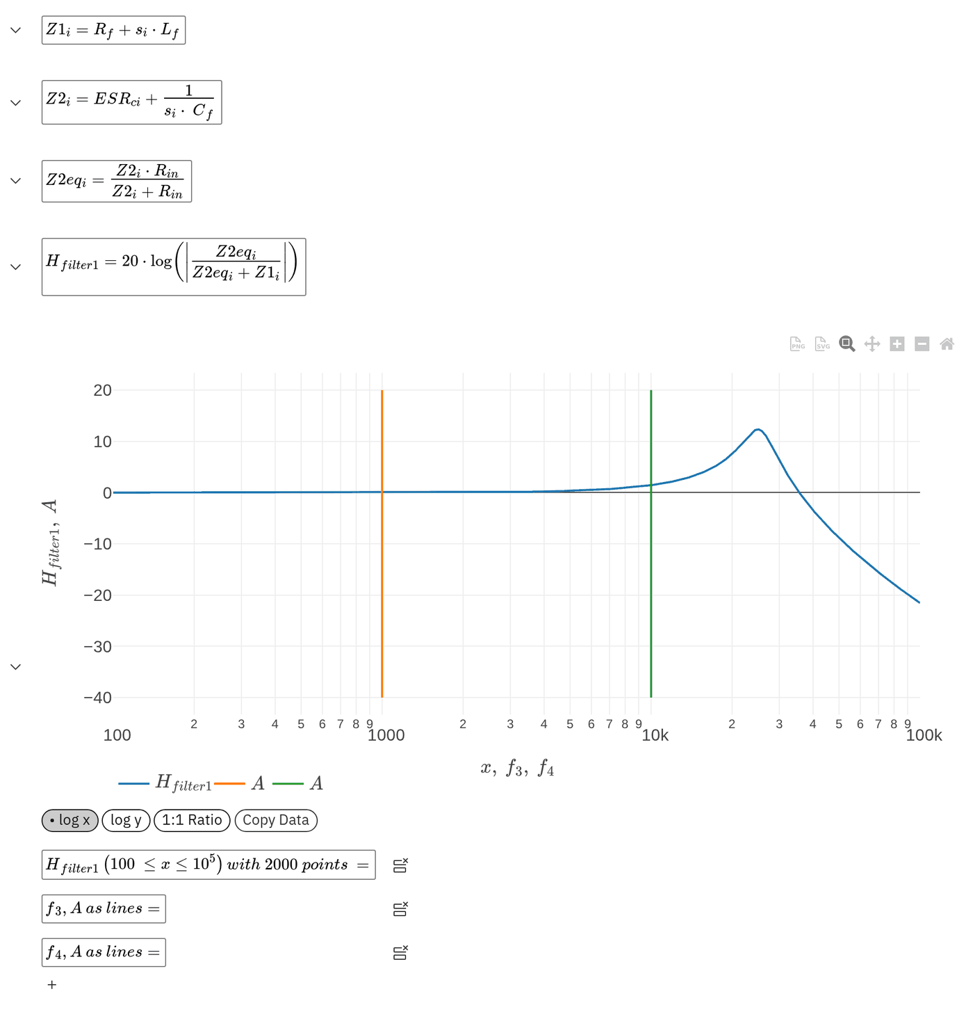
All the figures below are screenshots of our actual sheet. A quick note on the plots: the sweep variable x is the angular frequency in rad/s. The sheet converts it with f = x / (2·π) and builds si = 2·π·i·f, where i is EngineeringPaper's imaginary unit. The vertical lines mark 1,000 and 10,000 rad/s.
1. Model the Converter's Input Impedance
The filter has to be designed against something, and that something is the converter's input impedance. We start with the note's buck-converter parameters: output voltage and current (as R0 = 5 Ω), the output inductor L0 and its resistance RL, the output capacitor C0 and its ESR, and the duty cycle D. Then we type in the note's input-impedance expression:
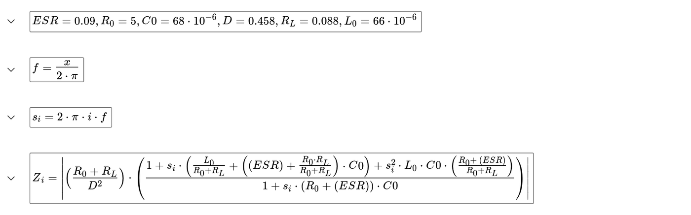
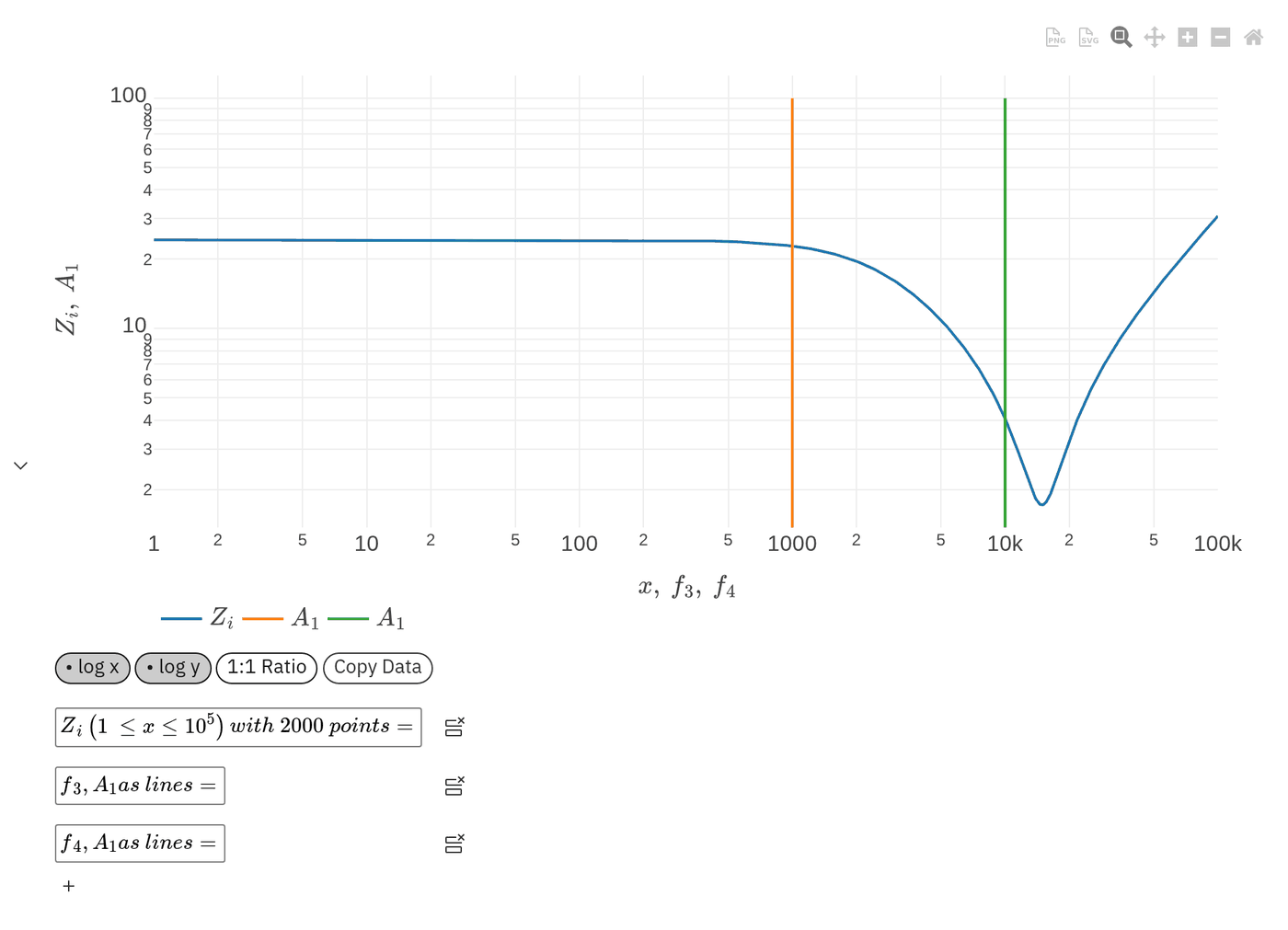
Because the sheet is live, sanity checks cost one line. At low frequency the impedance should approach (R0 + RL) / D2:

2. First-Pass LC Values
The converter rejects input noise below the crossover frequency of its control loop, 32 kHz in this example. Above that, the filter has to do the work. The note suggests placing the filter's corner well below the loop bandwidth and picks fc = 5 kHz. With the converter's 15 µF input capacitance, the required inductance and the damping factor follow:
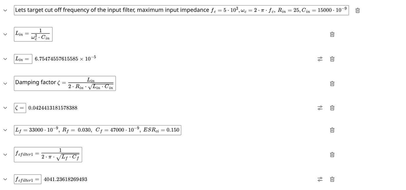
Every number matches the application note: 0.068 mH, ζ = 0.042 and 4.041 kHz. That line-by-line match is the moment we trust the sheet enough to change things.
Red flag: a damping factor of 0.042 is far below the 1/√2 ≈ 0.707 the note recommends as a good compromise. An undamped filter will peak hard at resonance.
3. Real Parts and the Transfer Function
With real parts, including the inductor's 30 mΩ resistance and the capacitor's 150 mΩ ESR, we build the impedances Z1i and Z2i, load the filter with Rin, and plot the transfer function:
4. The Middlebrook Stability Check
Middlebrook's extra element theorem gives the rule that matters most: the filter won't disturb the converter's control loop as long as the filter's output impedance stays well below the converter's input impedance at every frequency. In the sheet that's two curves on one plot:
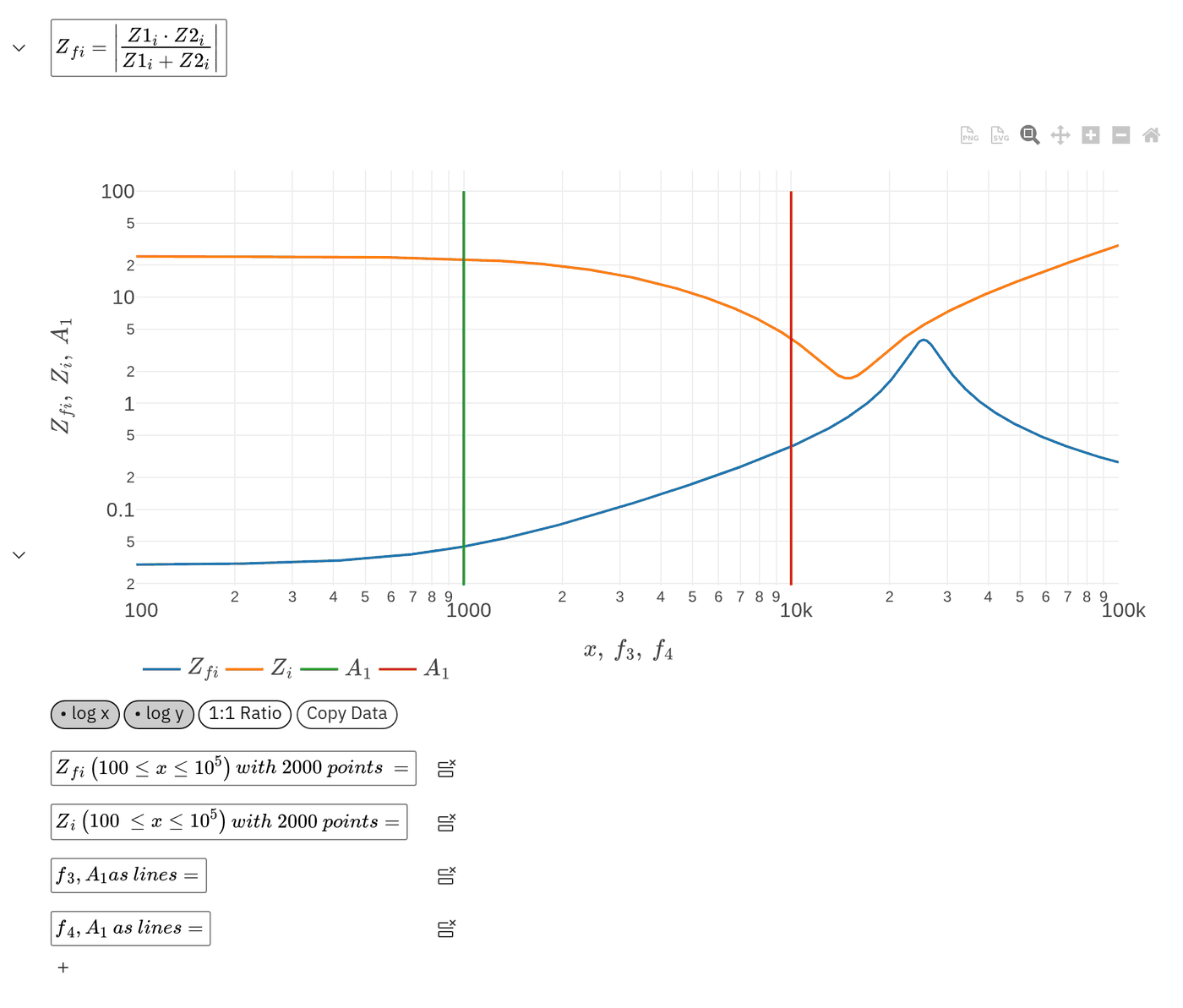
At its closest point, the converter's impedance is only about 1.35 times the filter's. That's far too close for comfort, once you allow for component tolerances, temperature and the converter's real closed-loop behavior. The filter needs damping.
5. Add Parallel Damping
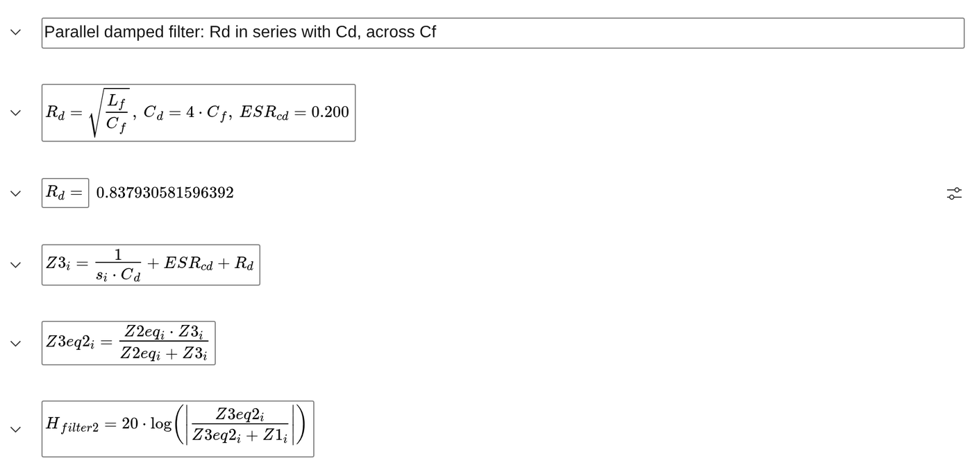
The note's parallel damped filter adds a resistor Rd in series with a blocking capacitor Cd, across the filter capacitor. Cd keeps DC out of Rd, so the resistor doesn't dissipate power. With Cd = 4·Cf, the note's optimum works out to Rd ≈ √(Lf / Cf). In the sheet that's five more lines:
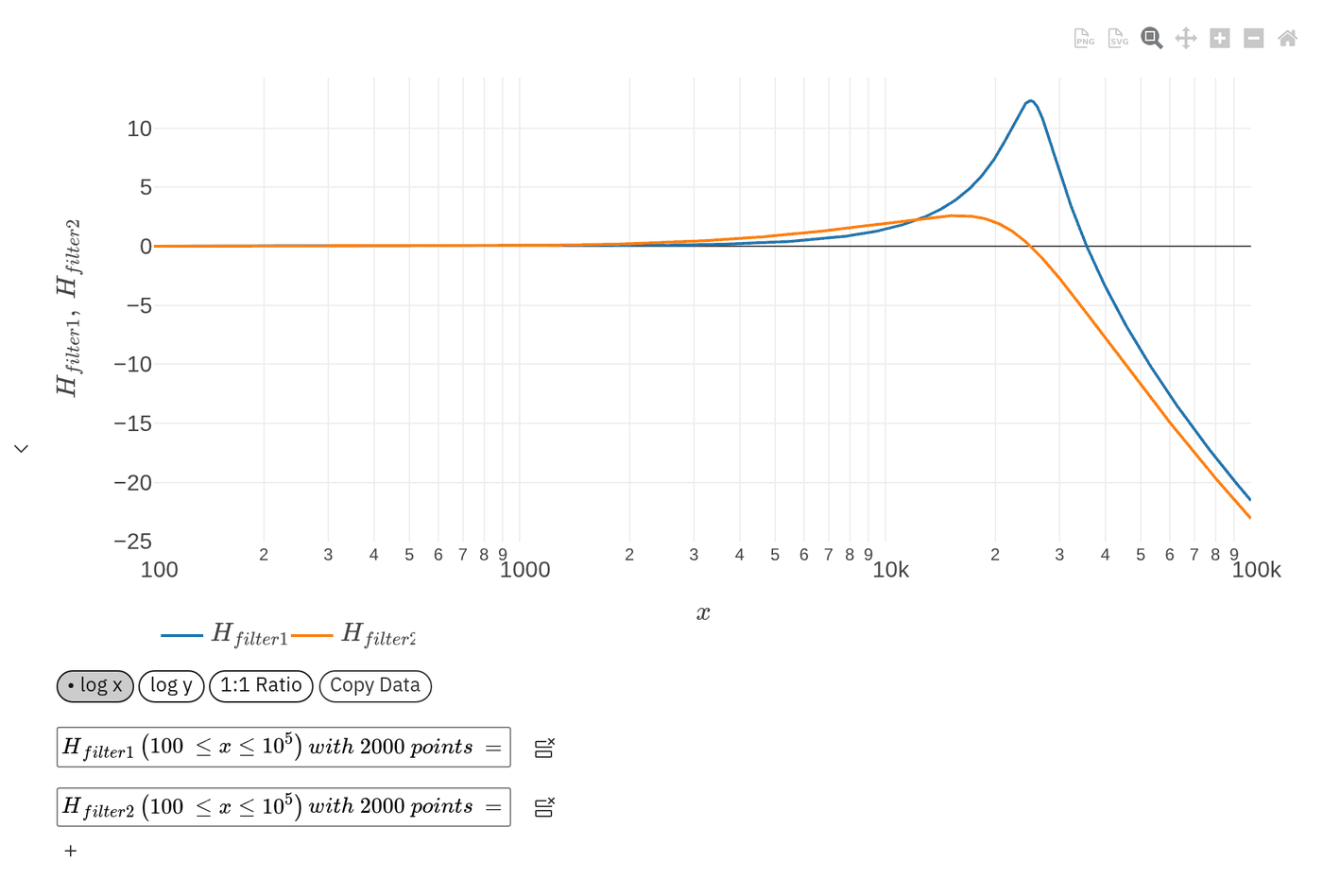
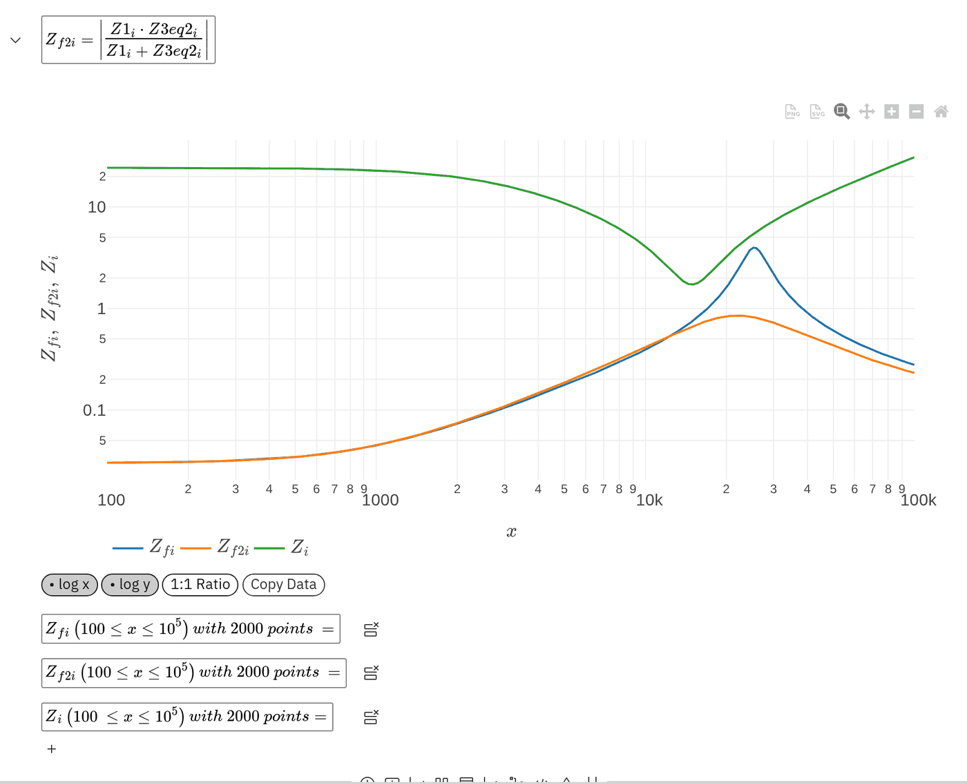
That's the result we were after: a filter that still attenuates the switching noise, about 43 dB at 100 kHz, and leaves a comfortable margin against the converter's input impedance.
Tips for Writing App-Note Math
- Copy names character for character. Use subscripts wherever the note does. When results disagree, you can find the line in seconds.
- Reproduce the note's numbers before you change anything. Our sheet matched 0.068 mH, 0.042 and 4.041 kHz before we touched a single value.
- Watch the complex frequency. s must be imaginary (s = i·ω). Using a real s gives a smooth curve with no resonance peak, which is exactly the problem you're trying to see.
- Watch rad/s vs. Hz. Application notes mix ω and f freely. Decide what your sweep variable is and label it.
- Add one-line sanity checks. DC limits, like (R0 + RL) / D2, catch typos before they reach a plot.
- Overlay before and after. Plotting the undamped and damped versions together makes design reviews much faster.
Where to Go From Here
The same sheet extends naturally to the rest of the application note:
- Series damping: Rd in series with Ld = n·Lf across the inductor. The note uses n = 2/15, so Ld = 4.4 µH.
- Two stages: the note's optimized ratios (L2 = 7·L1, C2 = 4·C1) reach about 80 dB of attenuation with a peak output impedance below 2 Ω.
- Component choice: pick capacitors with low ESL, and enough ripple-current rating. Splitting one capacitor into several in parallel lowers both ESR and ESL. For the inductor, keep the input and output leads apart and prefer single-layer or banked windings to reduce parasitic capacitance.
The sheet is where the design starts, not where it ends. The result still needs to be confirmed on the bench, for example by measuring the converter's input impedance or running a pre-compliance conducted-emissions scan.
Conclusion
Input filters are easy to get almost right, and "almost" means oscillation. TI's SNVA538 gives a clear method: model the converter, size the filter, check Middlebrook's criterion and damp the resonance. EngineeringPaper.xyz lets us follow that method with the note's own names and equations, check every number against the note, and see the impedance curves immediately. When a formula on paper looks like the formula on screen, reviewing a design takes minutes instead of an afternoon.